Reflective vs Formative

When finished, this page will explain using umx to make latent variables

Until now, to keep things simple as we learn, We have only had measured variables (boxes) on the diagram.

Of course, much of the power (and struggle) with SEM comes from the ability to use latent traits. These are represented on the diagram as circles. Conceptually, they are constructs that our theory postulates exist and which explain the state of our measured variables.

So, just like physicists never directly see electrons (and this lead some positivists to deny the validity of atomic theory), so to we never see things like extraversion: We only see behaviors – like a person being the centre of attention at a party, and we attribute these to our un-seen causal construct, extraversion. This is a powerful value of latent trait modelling: we are building causal models to explain what we see, not merely describe it. Extraversion then needs to be broken down into causal components and mechanisms which explain the desire to go to a party, whether we like most people we meet etc.

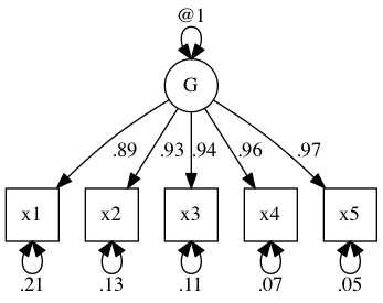
A simple example of building a latent variable exists on the fron page of the OpenMx website. Here it is:

require(umx)
data(demoOneFactor)
latents   = c("g")
manifests = names(demoOneFactor)
myData    = mxData(cov(demoOneFactor), type = "cov", numObs = 500)
m1 <- umxRAM("OneFactor", data = myData,
	umxPath(latents, to = manifests),
	umxPath(var = manifests),
	umxPath(var = latents, fixedAt = 1)
)
umxSummary(m1, showEstimates = "std")
plot(m1)

Scale

You’ll have noticed I fixed the variance of g at 1. This is known as giving a scale to the model. The reason we have to give some scale to the model is pretty simple: A path of 1 from a latent with variance 1 is the same as a path of .5 from a latent with variance .5. So, you can see, there are an infinite number of ways of fitting the same model which are equivalent. The optimiser can’t decide on one being better than another and so the solutions are unstable. By forcing the latent to take unit variance, we get a unique fit.

An alternative method you will see used widely, but which I don’t prefer is equally valid: To set the value of one of the paths.

Let’s do that to compare:

m2 <- umxRAM("FixedPath", data = myData,
	umxPath(latents, to = manifests, firstAt = 1),
	umxPath(var = manifests),
	umxPath(var = latents)
)
umxCompare(m1, m2)

This shows us the umxPath “firstAt” parameter in use. This sets the fist value in a list of paths to some value, in this case 1.

umxCompare shows us that both these methods provide equal fit. The difference comes in interpreting the paths.

Reflective and Formative constructions

It is as valid to think of our latent construct as being formed from certain inputs (perhaps five independent genes that all increase extraversion). Let’s do that:

m3 <- umxRAM("formative", data = myData,
	umxPath(manifests, to = latents),
	umxPath(var = manifests, fixedAt = diag(var(demoOneFactor))),
	# umxPath(var = manifests),
	umxPath(unique.bivariate = manifests),
	umxPath(var = latents, fixedAt=0)
)
plot(m3)
    

Reflective

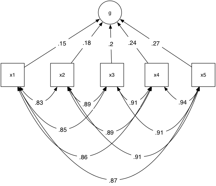
As you can see, we had to let the manifest variables covary among each other. This shows you the nifty umxPath “unique.bivariate” parameter that makes this a 1-line task.

There are a range of issues with treating latent variables as reflective variables. The most important in my mind is that the covariance structure of the measures themselves can vary and this will alter what the formative variable reflects.

umx!