Mendelian Randomisation and Instrumental Variables in umx
Instrumental variable (IV) analyses are widely used in fields as diverse as economics, and genetic epidemiology.
This page shows how to implement these analyses in umx.
IV analyses allow the estimation of causal relationships when confounding is likely but controlled experiments are not feasible. This ubiquitous situation has lead to many non-replicable findings driven by unmeasured or excluded confounders (Ioannidis, 2012).
Motivation: linear regression can be misleading
Consider some explanatory equation e.g. Y ~ 𝛽₁X + ε. As a scientific construct, this is interpreted as the causal claim that X plays a causal role in Y. Methodologically, we seek to create conditions that allow us to validly interpret significant estimates of 𝛽₁ as support for a causal role of X If, however covariates are correlated with the error terms, ordinary least squares regression produces biased and inconsistent estimates.[2]
Such correlation with error occurs when:
- The DV (Y) causes one or more of the covariates (“reverse” causation).
- One or more explanatory variables is unmeasured.
- Covariates are subject to measurement error.
Of course one or more of these are almost inevitable, making regression results suspect and often misleading.
If an instrument is available, these problems can be overcome. An instrumental variable is a variable that does not suffer from the problems of the confounded predictor. It must:
- Not be in the explanatory equation.
- Controlling for (“conditional on”) any other covariates, it must correlate with the endogenous explanatory variable(s).
In linear models, there are two main requirements for using an IV:
- The instrument must be correlated with the endogenous explanatory variables, conditional on the other covariates.
- The instrument cannot be correlated with the error term in the explanatory equation (conditional on the other covariates)
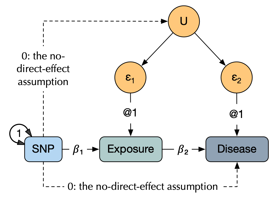
In this example, we examine the causal influence of X on Y, using an instrumental variable (qtl) which affects only X, based on Professor David Evans’ presentation at the 2016 International twin workshop,
The next block of code simply sets up a simulated dataset containing X, Y, qtl (a SNP affecting exposure X), and U - a covariate which induces a correlation between X and Y and which, if not measured, confounds the association of X and Y, allowing an errant researcher to assert evidence that X affects Y.
Our first analysis one is a simple linear model (or ordinary least squares regression). This will reveal a large association of X with Y and is the kind of analysis that has been criticised in false-positive epidemiology.
library(umx)
df = umx_make_MR_data(nSubjects = 10000, Vqtl = .02, bXY= .1, bUX= .5, pQTL= .5, seed = 123)

m1 = lm(Y ~ X    , data = df); umxAPA(m1) # Appears Y is caused by X:  β = 0.35 [0.33, 0.37]
m1 = lm(Y ~ X + U, data = df); umxAPA(m1) # Controlling U reveals the true link: β = 0.09 [0.07, 0.11]
Mendelian randomization analysis
Next, we analyse a Mendelian randomization trial.
A conventional implementation involves two-stage least squares. In R, we can do this using John Fox’s tsls function from the from sem library
m1 = sem::tsls(formula = Y ~ X, instruments = ~ qtl, data = df); coef(m1)
summary(m1)
| Estimate | Std. | Error | t | |
|---|---|---|---|---|
| (Intercept) | 0.002 | 0.010 | 0.238 | 0.812 |
| X | 0.159 | 0.075 | 2.108 | 0.035 |
Now we can see that X may indeed affect Y, but with the simulated effect size now correctly estimated at .1 (as specified in the simulated data) rather than the confounded .35 reported from the simple lm previously presented. Importantly, we didn’t need to know (measure) U, (the confounders).
Implementing MR in umx
You could of course build an MR model with umxRAM, but umx also gives us the shortcut umxMR function which builds the model for you.
First, umxRAM:
df = umx_make_MR_data(10e4)
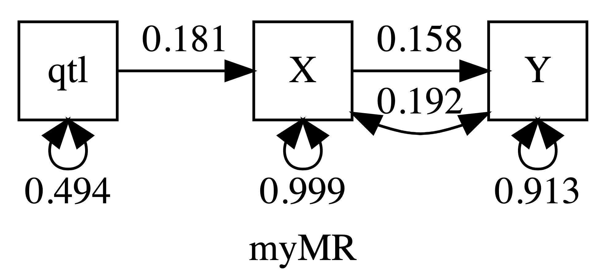
m2 <- umxRAM("myMR", data = df, autoRun = FALSE,
umxPath(v.m. = c("qtl", "X", "Y")),
umxPath("qtl", to = "X"),
umxPath("X", to = "Y")
# umxPath("X", with = "Y") # Due to OpenMx rules, will be deleted!
)
m2 <- umxModify(m2, "X_with_Y", free = TRUE, value = .2)
note: This double-step is required because OpenMx will otherwise over-write the X→Y path when you add X↔Y.
plot(m2, digits = 3)
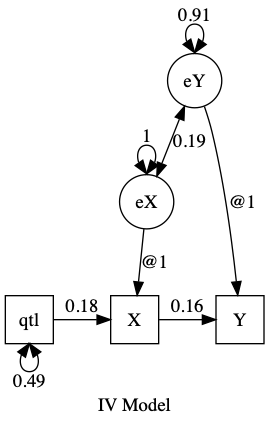
umxMR
Now an exactly equivalent model in umxMR:
df = umx_make_MR_data(10e4)

m1 = umxMR(Y~X, instruments= ~qtl, data = df)

plot(m1, means = FALSE, min = "")
TODO:
- Add an example with data in which the assumptions are violated, e.g.
qtldirectly affectsY, or affectsU
Refs Ioannidis, J. P. (2012). Why Science Is Not Necessarily Self-Correcting. Perspectives in Psychological Science, 7, 645-654. doi:10.1177/1745691612464056