plotting

TODO: Update for the ability to control plot layout with same, spline, max

“The plot thickens”

If you’ve used R, you’ll be used to plot for graphical output. With umx, plot works for umxRAM and twin (umxACE etc.) models!

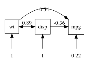
Just plot(model), and you will get a path diagram displayed in your browser (or RStudio graph window if you use RStudio). We’ll learn later how to open plots in other applications (like Graphviz), including for editing in apps like OmniGraffle).

m1 = umxRAM("cars", data = mtcars, type="cov",
	umxPath(c("wt", "disp"), to = "mpg"),
	umxPath("wt", with = "disp"),
	umxPath(var = c("wt", "disp", "mpg"))
)
plot(m1)

plot writes a “dot” file. This is another Bell Labs invention (just like R’s predecessor “S”) to specify “graphs” -for our purposes, objects (nodes) linked by lines (“edges”)- and lay them out (not an easy problem). By default, it opens courtesy of Richard Iannone’s fabulous DiagrammR package.

Inside a Graphviz file

Just so you know what we are working with, here’s the .gv file for the model above:

digraph G {

	mpg  [shape = square];
	wt   [shape = square];
	disp [shape = square];
	mpg_var  [label="0.22", shape = plaintext];
	wt_var   [label="1",    shape = plaintext];
	disp_var [label="1",    shape = plaintext];

	# Single arrow paths
	wt   -> mpg [label="-0.54"];
	disp -> mpg [label="-0.36"];

	# Variances
	mpg_var  -> mpg;
	wt_var   -> wt;
	wt       -> disp [dir=both, label="0.89"];
	disp_var -> disp;

	{rank = same; mpg wt disp};
	{rank = max ; mpg_var wt_var disp_var};

}

You can manually edit this (it’s just text) to get a different layout.

On Mac, plot will open this file in your default app for .gv files. I set this to graphviz.

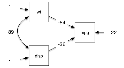
On MacOS Omnigraffle can open .gv files, and allows awesome publication-quality graphics.

So we can make the above example into this in about 1 minute (I timed it):

Parameters for plot.MxModel()

The parameters of plot give you a lot of flexibility. You can set the name of the file (it defaults to the model name), show unstandardised output, set the rounding for loadings, choose to show labels rather than estimates of paths, show or hide fixed paths, and means, and error variance.

plot(model, std = F, means = T, digits = 2, file = "name", ...)

More advanced controls include showing labels, not showing fixed paths, or modifying how residuals are drawn with resid = c("circle", "line", "none")

These are described below.

Standardized output and digit rounding

You can optionally output standardised output using std = TRUE, and control the number of values after the decimal with digits = (as well as strip_zero = TRUE to strip off leading “0.” from parameter values - can be helpful for cluttered figures).

plot(m1, std = TRUE, digits = 3, strip_zero = TRUE)

Plot style: residuals, means, fixed paths

The correct way to draw a residual is a double headed arrow from an object back to the object. This is the default for plot.

Omnigraffle doesn’t import or allow you to edit these easily, so for omnigraffle editing, you might switch to resid = “line”.

For clarity you can turn this off all together with resid = "none". You can also suppress drawing means, and turn on drawing fixed paths as you choose.

resid = c("circle", "line", "none")
fixed = FALSE, 
means = FALSE,

You can control how lines are drawn with the “splines” option. Users can also force the plot engine to group sets of variables at the top (min=), same or bottom (max) of the plot, which helps layout complex models.

File output and filename

The path model can be written to a file (the default is the name of the model with “.gv” suffix.

Don’t write any file

plot(m1, file = NA)

Override the default name

plot(m1, file = "my nice example") 

Give a full file path

plot(m1, file = "~/tmp.gv") # specify a file

TODO: tutorial on umx_set_plot_file_suffix and umx_set_plot_format

TODO: examples for same and spline parameters.