Getting Started: Build & run your first SEM model
I called this post “first steps” but it will take you a long way into practical modeling. Let’s go…
If you haven’t installed umx, do that now, and follow the link back here.
# load umx library
library("umx")
note: umx ? function help is not just boilerplate documentation: All functions have real-world examples to build on!
Overview
For those of you who like to get straight to the code: on this page we will build up a simply one-group structural equation model.
m1 = umxRAM("gas mileage", data = mtcars,
	# One headed paths from engine displacement and vehicle weight to miles/gallon
	umxPath(from = c("disp", "wt"), to = "mpg"),
	# Allow predictors to covary
	umxPath("disp", with = "wt"),
	# Freely estimate variances and means for each manifest
	umxPath(v.m. = c("disp", "wt", "mpg"))
)
umxSummary(m1, std = TRUE)
umxSummary table of model 1
| name | Std.Estimate | Std.SE | CI |
|---|---|---|---|
| disp_to_mpg | -0.36 | 0.18 | -0.36 [-0.71, -0.02] |
| wt_to_mpg | -0.54 | 0.17 | -0.54 [-0.89, -0.2] |
| mpg_with_mpg | 0.22 | 0.07 | 0.22 [0.08, 0.35] |
| disp_with_disp | 1.00 | 0.00 | 1 [1, 1] |
| disp_with_wt | 0.89 | 0.04 | 0.89 [0.81, 0.96] |
| wt_with_wt | 1.00 | 0.00 | 1 [1, 1] |
χ²(87) = 0, p < 0.001; CFI = 1; TLI = 1; RMSEA = 0
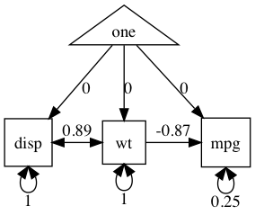
Now, we can update this model by dropping the path from displacement to mpg.
Note: umxRAM auto-labels all paths based on what they do like this: “disp_to_mpg”
m2 = umxModify(m1, update = "disp_to_mpg", name = "drop effect of capacity", comparison = TRUE)
umxCompare model 1 2
| Model | EP | Δ -2LL | Δ df | p | AIC | Compare with |
|---|---|---|---|---|---|---|
| gas mileage. | 9 | 419.1183 | ||||
| drop effect of capacity | 8 | 3.8616447 | 1 | 0.049 | 420.9800 | gas mileage |
And plot this model:
plot(m2)
Now, let’s go into more detail on the build, run, summarize, modify/compare, and display options step by step.
Two theories to compare
Here, we begin with a simple prediction in a built-in dataset: miles/gallon (mpg) goes down linearly with increases in car mass car and as engine size (capacity) goes up. Our contrasting theory predicts that “only weight matters”, not engine capacity. We can compare these claims by building model 1, then dropping capacity and testing if this model fits significantly worse.
We will use the built-in mtcars data set. miles/gallon is mpg, displacement is disp, and weight is wt.
note: mtcars + Henderson & Velleman’s (1981) “Building Multiple Regression Models Interactively” can teach you a lot of statistics in a very short period of time: Recommended!
Building on what you already know
In lm, model 1 would be mpg ~ disp + wt. Model 2 would be mpg ~ disp and you might compare them with anova(m1, m2)
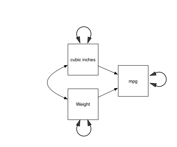
Sewall Wright invented SEM to allow us to think in explicit graphs specifying the model with both complete mathematical precision and easy graphical intuition. In Wright’s terms, the model we are describing is shown in the figure below as “A model of Miles/gallon”
Your first umxRAM model
The umx equivalent of lm is umxRAM, and we build the “formula” using umxPaths. Something very simple: the means and variances of three raw variables. This is also called an “independence model”.
We feed this model-container a data set the way that most R models use: (data = mtcars).
m1 = umxRAM("my_first_model", data = mtcars,
	umxPath(var   = c("disp", "wt", "mpg")),
	umxPath(means = c("disp", "wt", "mpg"))
)
These two steps of giving a variable a variance and a mean are so common, umx has a shortcut "v.m." =
m1 = umxRAM("independence_model", data = mtcars,
	umxPath(v.m. = c("disp", "wt", "mpg"))
)
Clearly some un-modeled covariance here… Let’s build our theorized model.
Next, we can add more umxPaths to specify all the arrows, boxes, and circles in the figure above.
note: umxPath has many shortcuts for specifying a path: So a list of variances (2-headed path originating and terminating on one variable) are set with the argument var =c(x, y, z)
To specify a mean (a path from the constant one to a variable), just use the argument means =. You can learn more about umxPath in the help and in this chapter on using umxPath.
Just like lm, umxRAM defaults to running the model automatically and it prints out a table of fit-information.
nb: You can re-run a model anytime with umxRun()
You can also request a summary, and plot the output:
umxSummary(m1)
plot(m1)
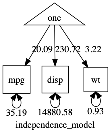
note: When you are running real models, having variances differ by orders of magnitude can make it hard for the optimizer. In such cases, you can often get better results making variables more comparable: in this case, for instance, by converting displacement into litres to keep its variance closer to that of the other variables. (see here for a post on renaming variables (like “disp” to “displacement”), and scaling variables/data-wrangling)
As you can see, this is an “independence model”: No covariances were included, so all variables are modeled as uncorrelated. It would fit poorly in this case. umxSummary tells us this fit can definitely be improved: χ²(90) = 98.32, p < 0.001; CFI = 0; TLI = 0; RMSEA = 0.996
This new model is better, i.e., the three degrees of freedom were worth paying for in improved fit to the data:
| Model | EP | Δ -2LL | Δ df | p | AIC | Compare with Model | |
|---|---|---|---|---|---|---|---|
| 1 | big and heavy | 9 | 419.12 | ||||
| 2 | independence_model | 6 | 98.312 | 3 | < 0.001 | 511.44 | big and heavy |
In fact this (saturated) model fits perfectly, as umxSummary shows: χ²(87) = 0, p < 0.001; CFI = 1; TLI = 1; RMSEA = 0
m2 = umxRAM("big and heavy", data = mtcars,
	# One headed paths from disp and weight to mpg
	# Allow predictors to Covary
	# Variances and Means
	umxPath(c("disp", "wt"), to = "mpg"),
	umxPath(cov = c("disp", "wt")),
	umxPath(v.m = c("disp", "wt", "mpg"))
)
We can drop the path by label:
m2 = umxModify(m1, update = "disp_to_mpg", name = "drop effect of capacity", comparison = TRUE)
You can compare models anytime with
umxCompare(m2, m1)
We can request a full summary including standardized output as a table with (“show = std” requests the standardized paths):
umxSummary(m2, std = TRUE)
| name | Estimate | Std.Error | CI (SE-based) | |
|---|---|---|---|---|
| 1 | disp_to_mpg | -0.37 | 1.8e-01 | -0.37 [-0.72, -0.02] |
| 2 | wt_to_mpg | -0.54 | 1.8e-01 | -0.54 [-0.89, -0.2] |
| 3 | mpg_with_mpg | 0.21 | 6.8e-02 | 0.21 [0.08, 0.35] |
| 4 | disp_with_disp | 1.00 | 1.9e-12 | 1 [1, 1] |
| 5 | disp_with_wt | 0.89 | 3.7e-02 | 0.89 [0.82, 0.96] |
| 6 | wt_with_wt | 1.00 | 2.5e-13 | 1 [1, 1] |
We can plot these standardized (or raw) coefficients on a diagram the way Sewell Wright would like us too:
plot(m2, means = FALSE) # plot has lots of control: here we suppress display of the means
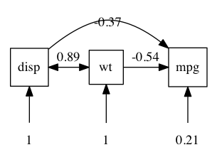
note: Means are not shown on this diagram (showMeans =FALSE) though they are in the model.
We can ask for the (unstandardized) confidence intervals with the usual confint function. Because these can take a long time for SEM models, the default is to require you to ask to run them.
confint(m2, run = TRUE)
| lbound | estimate | ubound | |
|---|---|---|---|
| disp_to_mpg | -0.035 | -0.018 | 0.000 |
| wt_to_mpg | -5.641 | -3.351 | -1.060 |
| mpg_with_mpg | 4.866 | 7.709 | 13.642 |
| disp_with_disp | 4536 | 15360 | 24081337 |
| disp_with_wt | 58.605 | 107.685 | 286.965 |
| wt_with_wt | 0.589 | 0.951 | 1.590 |
| one_to_mpg | 30.631 | 34.960 | 39.291 |
| one_to_disp | 173.627 | 230.815 | 287.822 |
| one_to_wt | 2.871 | 3.218 | 3.560 |
What did lm think these should be?
l1 = lm(mpg ~ 1 + disp + wt, data = mtcars)
coef(l1)
| (Intercept) | disp | cyl |
|---|---|---|
| 34.96055404 | -0.01772474 | -3.35082533 |
confint(l1)
| 2.5 % | 97.5% | |
|---|---|---|
| (Intercept) | 30.53357368 | 39.387534392 |
| disp | -0.03652128 | 0.001071794 |
| wt | -5.73173459 | -0.969916079 |
Next, we can modify and compare this model, with one in which only weight affects mpg.
Modify and Compare models: The secret-sauce of science
In graph terms a question like “does lower weight give better miles per gallon” is asking, “can I set the path from wt to mpg to zero without significant loss of fit?”
There are two ways to test this with umx.
First, we can modify m2 by overwriting the existing path with one fixing the value to zero.
With umxPath we can save some typing and use fixedAt
m3 = umxRAM(m2, umxPath("disp", to = "mpg", fixedAt = 0), name = "weight_doesnt_matter")
As you develop skill with umx, you ‘ll often umxModify a model, instead of building a whole new model
m3 = umxModify(m2, update = "disp_to_mpg", name = "weight_doesnt_matter")
That examines our competing theoretical prediction, with a “zero” path from wt to mpg (weight of car to fuel economy)
Compare two models
Now we can test if weight affects mpg by comparing these two models:
umxCompare(m2, m3)
As you develop skill with umx, you might umxModify and compare in one step:
m3 = umxModify(m2, update = "disp_to_mpg", name = "weight_doesnt_matter", comparison = TRUE)
The table below shows that dropping this path caused a (just) significant loss of fit (χ²(1) = 3.96, p = 0.049):
| Model | EP | Δ -2LL | Δ df | p | AIC | Compare with Model |
|---|---|---|---|---|---|---|
| big and heavy | 9 | 419.13 | 419.12 | |||
| weight_doesnt_matter | 8 | 3.86 | 1 | 0.049 | 420.98 | big and heavy |
The AIC moved the wrong direction, p-value is marginal. This model would lead us to conclude that weight matters, but would prompt us to do controlled experiments varying weight and looking for confounders like aerodynamic drag.
Note however that these variables covary: heavy vehicles have big motors: This is why trying to do science on observational data is fraught with problems. MUCH better to systematically vary the weight in a randomized controlled trial and measure mpg change. In behavior science, Twin Studies and Mendelian Randomization let us do this.
Advanced tip: umxModify() can modify, run, and compare all in 1-line. For instance to drop the path from wt to mpg, we can say:
m4 = umxModify(m2, update = "wt_to_mpg", name = "drop effect of wt", comparison = TRUE)
You will use umxModify often.
By default, umxModify fixes the value of matched labels to zero. Learn more at the umxModify tutorial.
tip: To discover the labels in a model, use parameters(model) (or just call umxModify with no update)
The umx version of parameters is on steroids - you can filter using wild card patterns! So
umxGetParameters(m3, pattern = "^mpg")
# [1] "mpg_to_mpg"   "mpg_to_disp"  "mpg_to_wt"    "mpg_with_mpg" "mpg_with_wt"