EFA (Exploratory factor analysis) using umx
Factor analysis takes a number of measured variables (manifest variables) and accounts for these in terms of a (smaller) number of latent variables, and uncorrelated residual variance, specific to each manifest variable. The number of factors to retain can be estimated using various methods including Horn’s parallel analysis. These factors define a multi-dimensional space within which the items are located. The factors themselves can be transformed (rotated) to a simpler structure.
Performing a factor analysis in R is straightforward, as long as one does not have missing data. This code snippet gives an example of an analysis of 5 variables from the ubiquitous mtcars data set, retaining 2-factors:
factanal(~ mpg + disp + hp + wt + qsec, factors = 2, rotation="promax", data = mtcars)
#      Factor1 Factor2
# mpg  -0.851   0.345
# disp  0.871  -0.356
# hp    0.621  -0.701
# wt    0.996
# qsec -0.123   0.906
In umx, we can replicate this analysis with the umxEFA function:
vars = c("mpg", "disp", "hp", "wt", "qsec")
m2 = umxEFA(name = "test", factors = 2, data = mtcars[, vars])
x = mxStandardizeRAMpaths(m2, SE= TRUE)
The loadings matrix is just:
load = m2$A$values[manifests, latents]

if rotation == "varimax"){
	load = varimax(load, normalize = TRUE, eps = 1e-5))
} else if (rotaions == "promax"){
	load = promax(load, m = 4)
}

m2$A$values[manifests, latents] = load
require(umx)

manifests = names(data)
m1 = umxRAM(model = name, data = data, autoRun = FALSE,
	umxPath(factors, to = manifests, connect = "unique.bivariate"),
	umxPath(v.m. = manifests),
	umxPath(v1m0 = factors, fixedAt = 1)
)

data(demoOneFactor)
latents   = c("g", "f")
manifests = names(demoOneFactor)
myData    = mxData(cov(demoOneFactor), type = "cov", numObs = 500)
m1 = umxRAM("f", data = myData,
	umxPath(latents, to = manifests, connect = "unique.bivariate"),
	umxPath(var = manifests),
	umxPath(var = latents, fixedAt = 1)
)

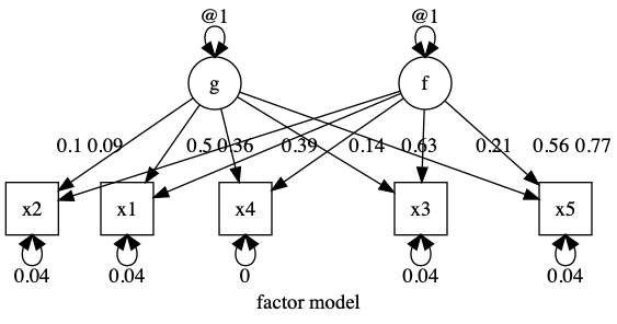
plot(m1, splines = FALSE)
| name | Estimate | SE |
|---|---|---|
| g_to_x1 | 0.090 | 2.759 |
| g_to_x2 | 0.101 | 3.535 |
| g_to_x3 | 0.139 | 3.992 |
| g_to_x4 | 0.360 | 4.523 |
| g_to_x5 | 0.207 | 5.456 |
| f_to_x1 | 0.387 | 0.639 |
| f_to_x2 | 0.496 | 0.717 |
| f_to_x3 | 0.560 | 0.991 |
| f_to_x4 | 0.634 | 2.569 |
| f_to_x5 | 0.765 | 1.474 |
| x1_with_x1 | 0.040 | 0.003 |
| x2_with_x2 | 0.035 | 0.003 |
| x3_with_x3 | 0.040 | 0.003 |
| x4_with_x4 | 0.000 | 0.071 |
| x5_with_x5 | 0.040 | 0.005 |
| g_with_g | 1.000 | 0.000 |
| f_with_f | 1.000 | 0.000 |
χ²(0) = 1.85, p = 1.000; CFI = 1; TLI = 1; RMSEA = 0