umx!

Twin ACE Cholesky with umxACE

The Multivariate ACE Cholesky is a core model in behavior genetics (Neale & Maes, 1996), and umx implements this as umxACE.

The ACE model decomposes phenotypic variance into Additive genetic (A), unique environmental (E) and, optionally, either common or shared-environment (C) or non-additive genetic effects (D). The latter restriction emerges due to a lack of degrees of freedom to simultaneously model C and D given only MZ and DZ twin pairs.

The Cholesky or lower-triangle decomposition ensure a model that is solvable, and also accounts for all the variance (with some restrictions) in the data. This model creates as many latent A C and E parameters as there are phenotypes, and, moving from left to right, decomposes the variance in each component into successively restricted factors (see Figure below).

Diagram	Matrix
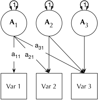	3 × 3 matrix-form of the Cholesky paths, with labels as applied by umxLabel. A1 A2 A3 Var 1 a_r1c1 Var 2 a_r2c1 a_r2c2 Var 3 a_r3c1 a_r3c2 a_r3c3
Multivariate ACE Cholesky model, showing the additive genetic component only (C and E take identical forms) and for one-twin only (each model in umxACE describes the A, C (or D), and E paths, constrained appropriately across the members of the pair, contingent on their zygosity.

Data Input

umxACE flexibly accepts either raw data or summary covariance data (in which case the user must also supply numbers of observations for the data sets). In an important capability, the model transparently handles ordinal (binary or multi-level ordered factor data) inputs, and can handle mixtures of continuous, binary, and ordinal data in any combination. In terms of loss function, FIML and WLS are supported. On the roadmap, is handling Tobit modeling.

umxACE also supports weighting individual data rows. In this case, the model is estimated for each row individually, then each row’s likelihood is multiplied by its weight, and these are summed to form the model likelihood (the target for the optimizer). This feature is currently used to implement non-linear umxGxE_window function.

In addition, umxACE supports varying the DZ genetic association (defaulting to .5) to allow exploring assortative mating effects, as well as varying the DZ “C” factor from 1 (the default for modeling family-level effects shared 100% by twins in a pair), to .25 to model dominance effects.

Interpretation and graphing

Models built by umxACE are able to be plotted and summarized using plot and umxSummary. umxSummary can report A, C, and E path-coefficients, along with model fit indices, and genetic correlations (Rg = TRUE). plot is extended by umx to handle graphical reporting of ACE models, laying out models as seen in Figure 2.

ACE Examples

We first set up data for a summary-data ACE analysis of weight data (using a built-in example dataset from Nick Martin’s Australian twin sample:

require(umx); data(twinData)
dz = subset(twinData, zygosity == "DZFF" & cohort == "younger")
mz = subset(twinData, zygosity == "MZFF" & cohort == "younger")

The next line shows how umxACE allows the user to easily build an ACE model with a single function call. umx will give some feedback, noting that the variables are continuous and that the data have been treated as raw.

We could conduct this same modeling using only covariance data, offering up suitable covariance matrices to mzData and dzData, and entering the number of subjects in each via numObsDZ and numObsMZ.

m1 = umxACE(selDVs = c("wt"), sep = "", dzData = dz, mzData = mz)

By default the model will run itself

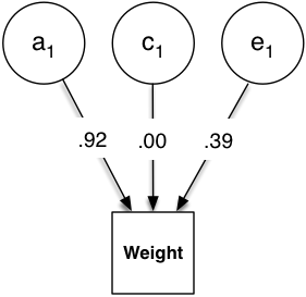
You can plot with:

plot(m1) # output shown below

umxSummary provides a summary table:

umxSummary(m1)

-2 × log(Likelihood) = 12186.28 (df = 4)

Standardized solution

By default the report table is written to the console in markdown-format. By setting report = “html”, the user can request a rendered html be opened in the default browser. Whether the parameter table is standardized or not is set using the showStd = TRUE parameter (the default). The user can request the genetic correlations with showRg = TRUE (the default is FALSE). If Confidence intervals have been computed, these can be displayed with CIs = TRUE.

The user can control the precision of output with the digits = parameter. The umxSummary function can also call the plot in line (file = "name"). More advanced features include that the function can also return the standardized model (returnStd = TRUE). A model fit comparison can also be requested by offering up the comparison model in comparison = model.

The help (?umxACE) for umxACE gives extensive examples, including binary, ordinal, and joint data setup and analysis.